Data Analytics Case Study – 2021
For this case study I analyzed data from 33 Fitbit users over the course of a 30-day period.
The goal of the project is to analyze smart device usage data in order to gain insight into how consumers use smart devices and apply this analysis to one product from Bellabeat, a high-tech company that manufactures health-focused smart products founded by from Urška Sršen and Sando Mur.
Sršen used her background as an artist to develop beautifully designed technology that informs and inspires women around the world. Collecting data on activity, sleep, stress, and reproductive health has allowed Bellabeat to empower women with knowledge about their own health and habits. Since it was founded in 2013, Bellabeat has grown rapidly and quickly positioned itself as a tech-driven wellness company for women.
One of Bellabeat’s product is Leaf. This wellness tracker created with Swarovski® crystals doubles as a jewellery piece that can be worn as a bracelet, necklace, or a clip. It tracks activity, sleep, menstrual cycle, stress sensitivity, and access other exclusive wellness content. This analysis will be applied specifically to Leaf and inform high-level recommendations for the marketing strategy.
Tracking Wellness Trends – Market Research
From GWI:
Globally, usage of health and fitness apps is on the rise. In 2012, 11% of internet users said they used a health and fitness app in the last month, rising to 26% in 2019 – a growth of 136%.
While millennials are using health apps the most (29%), baby boomers aren’t too far behind (19%) – highlighting that health apps, regardless of age, allow users to take more control over their health through the devices they use every day.
Additionally, from recent custom coronavirus research across 17 countries between March 31st-April 2nd, maintaining physical wellness is vital for consumers at this time.
Globally, around 1 in 5 internet users now own a smartwatch or smart wristband; a 46% increase since 2014.
In separate custom research from early March in the U.S. and UK, 3 in 5 smartwatch/fitness tracker owners use their wearable for step counting.
For example, 44% of smartwatch/fitness tracker owners use their device to measure or track their heart rate and 40% use it to track their sleep, while 27% use it for blood pressure measurement.
Younger audiences tend to use their wearables for a greater number of functions compared to Gen X and baby boomers who primarily use it for step tracking or tracking their heart rate.
Interestingly, 45% say they enjoy looking at the data, highlighting consumers’ need for more information, which is something many have become accustomed to in the age of digital sharing.
Additionally, around 40% of current/future wearable owners also want the ability to manage sleep-related issues, track their breathing rate, and manage stress issues – highlighting just how this technology is giving people the ability to quantify their physical and mental wellbeing through lifestyle changes and rituals.
Around 1 in 5 females in the U.S./UK say they use their smartwatch/fitness tracker for female health tracking – making this a more popular feature than diet tracking and stress relief.
From an article in the Washington Post:
“Fitbit is moving aggressively to sign up companies. It added a call service that will reach out to individual workers — via text messages and phone calls — whose data shows they are falling short of their fitness goals. It’s part of a concerted effort to improve the health of entire workforces.”
Problems with Wellness Trackers
From the study Analysis of Health Consumers’ Behavior Using Self-Tracker for Activity, Sleep, and Diet,:
“Analysis indicated that the ease of use of a particular device stands as the most significant barrier in the way of increasing the efficacy of self-tracking. Until the technological advances that allow automatic health data collection without user intervention reach a critical maturity level, the accuracy and reliability of logged data depend largely on an individual consumer’s attitude and behavioral intention. This is because health and biometric self-tracking is given an appropriate significance only when coupled with the consumer’s efforts and desires to be informed.”
From Wellsteps.com:
“Previous users of wearable devices have complained that they are easy to lose, they break, they’re really not waterproof (despite manufacturer’s claims), they are sometimes are difficult to sync with your smart phone, the batteries don’t last long enough, some of them are not very attractive, they may be uncomfortable to wear, and, at the end of the day, they don’t provide much material benefit.
Many of you reading this blog have a wearable device. Most people who have a wearable device are already quite fit, younger than average, and have a higher socioeconomic status than average. Most people stop using them after 12 months.”
From GWI:
Privacy factors are also key concerns. Around 1 in 5 millennials, Gen X, and baby boomers don’t want their health data to be accessible by others – compared to just 7% of Gen Z.
Gen X (18%) and baby boomers (16%) are also more wary about trusting the consistency or accuracy of the data than Gen Z (5%) or millennials (12%). In the UK, 24% of non-wearable owners say they don’t want to rely too much on technology compared to 17% in the U.S.
As might be expected, the cost of wearables was more of a deterrent for consumers in the lowest income bracket (46%). However, even among those in the top income bracket, 37% say the devices are often too expensive.
Opportunities for Bellabeat
Based on the global trends, Bellabeat is well-positioned to capture a percentage of the increasing popularity of wellness trackers.
Differentiators that Bellabeat’s Leaf product can really emphasize are:
-
- Leaf is stylish and feminine whereas most fitness trackers are bulky and plastic and do not mesh with more formal or business-style attire.
- Leaf offers a 6-month battery life so there is not a need to re-charge every few days.
- Leaf can also be worn as a bracelet, necklace or clip which makes it easier to consistently wear the device even when sleeping.
- Leaf runs on Bellabeat proprietary tracking technology developed to work for women’s bodies.
- The Leaf is made from a wood-composite material and hypoallergenic stainless steel clip (good for the environment).
- Leaf is set at an affordable price range of $89-$149.
- The data is owned and managed by Bellabeat.
Bellabeat’s current marketing strategy
Currently, Bellabeat products are available through a growing number of online retailers in addition to their own e-commerce channel on their website. The company has invested in traditional advertising media, such as radio, out-of-home billboards, print, and television, but focuses on digital marketing extensively. Bellabeat invests year-round in Google Search, maintaining active Facebook and Instagram pages, and consistently engages consumers on Twitter. Additionally, Bellabeat runs video ads on Youtube and display ads on the Google Display Network to support campaigns around key marketing dates.
How can Bellabeat better position Leaf?
Based on the research, there is a growing need for wellness trackers beyond fitness. Areas such as stress, sleep and menstruation are becoming more popular. People want to use these devices holistically, rather than just a fitness, steps or exercise tracker.
Wellness is the key word here, and targeting women who are struggling with health and weight issues could be a good market. By providing more insights into overall health data (sleep, menstruation, stress), Bellabeat can offer a more holistic wellness product combined with their subscription health advice.
Cost is a barrier, but Bellabeat’s products are well below the price of Garmin, Apple, etc.
Privacy of data is another core issue for users. Looking at Bellabeat’s website, there is no direct mention of how the data is collected and stored. This should be addressed.
Instead of mass marketing, focus on niche websites and magazines for women and style magazines such as Vogue, InStyle, People, etc. as well as wellness ambassadors and influencers (specifically the Millennial market as this age group is showing the largest growth). More personal stories of how the device works and has specifically improved health will be more effective than mass market campaigns.
The question for consumers should always be: how will understanding my health data improve my life? Give women information and explain how. To sell to women, you need to make an emotional connection. Word-of-mouth and social media performs very well in this market.
Also, when I do a google search of “wellness trackers women” Bellabeat is not mentioned in any articles. Perhaps, case studies (PR campaign) could also tell the story of how wearing Bellabeat Leaf has improved quality of life?
Also, the type of tracking offered is not communicated. Looking at the Fitbit data, users did not perform well when they had to manually input data. What types of auto-collected data does Bellabeat collect? How accurate is Bellabeat’s data? How can users apply Bellabeat’s data to their lives to improve their health and wellness? The simpler it is to capture the data, the more satisfied the user.
Data Summary
From the data, we can clearly see basic correlations: the amount of activity and the intensity of activity has a direct effect on calories burned and heart rate. We can also see some overall weekly trends, such as high activity on Tuesday and Saturday and low activity on Sunday and Wednesday.
We can also tell from the weight and BMI data, that longer distances and increased active minutes is attributed to users with higher BMI and weight, but is manually inputted so it was only entered by eight users. Sleep data shows that no users slept more than eight hours and this data is also unreliable as many users did not wear their Fitbit at night. Overall, device usage decreased over the 30-day period.
Looking at this data, Bellabeat is well positioned to market the Leaf device as easy-to-wear with a battery-life of six months. This ease and versatility of wear (as a bracelet, necklace or clip) combined with the battery life, would most likely mean that users would record more consistent and reliable data (such as sleep). Also, the more automatic data Bellabeat can capture the better as we can see from this dataset, users were unlikely to manually track their weight.
Bellabeat can also use this data to further incentivise users to get more sleep, maintain regular activity and accurately monitor weight/BMI.
Analyzing Fitbit Data
Step One: Prepare
For the capstone project, Google supplied a dataset of 33 FitBit users. The goal is to analyse this dataset and determine smart device usage data in order to gain insight into how consumers use non-Bellabeat smart devices.
Thirty-three eligible Fitbit users consented to the submission of personal tracker data, including minute-level output for physical activity, heart rate, and sleep monitoring. It includes information about daily activity, steps, and heart rate that can be used to explore users’ habits. The data included in this project contained a database with 18 files.
As the dataset only contains 33 users it is far from comprehensive. Looking through the data, not all users reported in each available file, for example only eight users are listed in the weight file.
As the data is from 2016, it is already five years old and therefore, not current. The data tracks 33 users over 30 days from 4/12/2016 to 5/12/2016 which is a very short window of time.
The data also has incomplete records which meant either the user did not wear their Fitbit or the data was not able to be collected. This makes the reliability of the data low.
Key demographics were not included with the data such as sex or age.
Step 2: Process
Cleaning the data involved understanding what data was included for the 33 users and if there is a complete set of data for all categories.
For example, since weight requires users to log their data, only eight users entered this data. Sleep was also not recorded consistently. Only one user actively captured all data.
The major inconsistencies were the date-times for users. Some entries were recorded as 24-hours, others were only entered as 12-hour. The time-date data was also imputed as text/string and required value formatting to be changed to consist of 24-hour date-time.
Many of the datasets were very large files and could only be opened in R Studio or Bigquery (SQL).
I began by exploring the data in Excel and Google Sheets. The files too large for Google Sheets were opened in Excel. Google Sheets easily formatted the date-time into 24-hours, but Excel required much more work to correctly format the date-time stamps.
Duplicates, errors and inconsistencies were not a major issue with the dataset.
The tools used to clean and analyze this data were: R Studio, Bigquery (SQL), Excel, Google Sheets and Tableau.
The steps, formulations, results and metadata can be found at the end of this page for further review.
Questions asked before analysis:
1. During which time of day were the users most sedentary? Most active? Why?
2. During which time of the week were the users most active? Most sedentary? Why?
3. What were the sleep trends? Which days had the most sleep minutes? Why?
4. Was there a correlation between steps and calories?
5. Was there a correlation between sleep and calories?
6. Is there a correlation between steps and sleep?
7. How did users report data? Automatically? Inputted?
8. User weak points? Strong points?
9. Why do some users have more data than others?
Step 3: Analyse
Fitbit User Snapshot
- Only 51% of users had an average of 20 minutes or more of active and fairly active minutes per day.
- Only 21% of users took more than 10,000 steps per day.
- An average of 78% of the user’s day is made up of sedentary minutes.
- An average of 20% of the user’s day is made up of fairly active minutes.
- Only 12% of users recorded an average of more than seven hours of sleep.
- Only 24% of users recorded an average of more than six hours of sleep.
- 27% of users did not record any sleep (did not wear their device at night).
- Only 24% of users recorded weight and BMI data.
- Average steps for all users: 7,652.
- Average hours of sleep for all users: 6.9 hours.
- Average weight for all users: 85.08kg/187.57lbs (only eight users recorded weight and BMI).
- Average BMI for all users: 24.89 (just inside the healthy weight range).
- Users are the most active between 5pm – 7pm daily.
Step 4: Share
Fitbit User Behaviours and Correlations
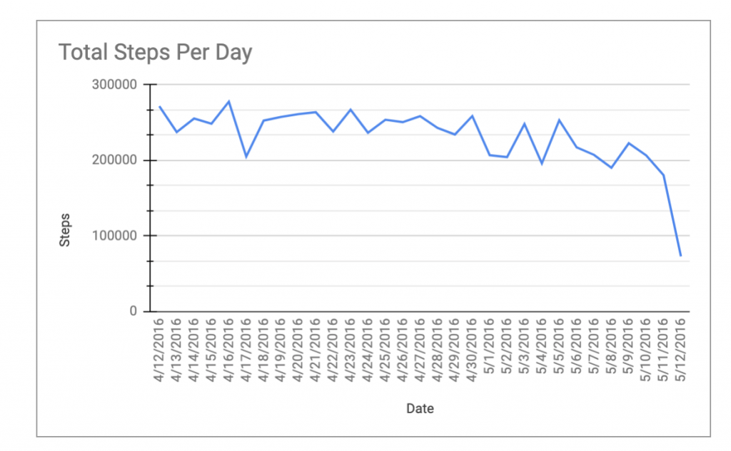
- Looking at the data overall, there was a negative correlation between device usage and time. For example, over the course of the 30-day period, user data decreased. This can be seen in the chart below in reference to total steps measured over the 30-day period. By 5/12/2016, the steps/ day is falling. Chart and calculations, Google Sheets.
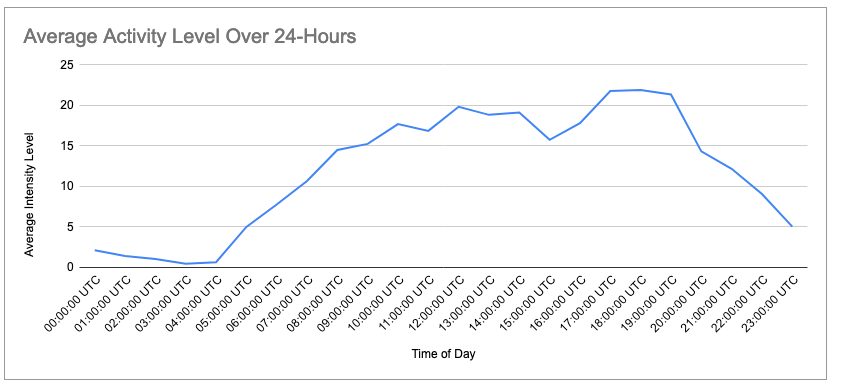
- There was a positive correlation between activity level and time of day for all users. Looking at the averages, most users were more active between the house of 5pm – 7pm. Chart and calculations performed in Google Sheets.

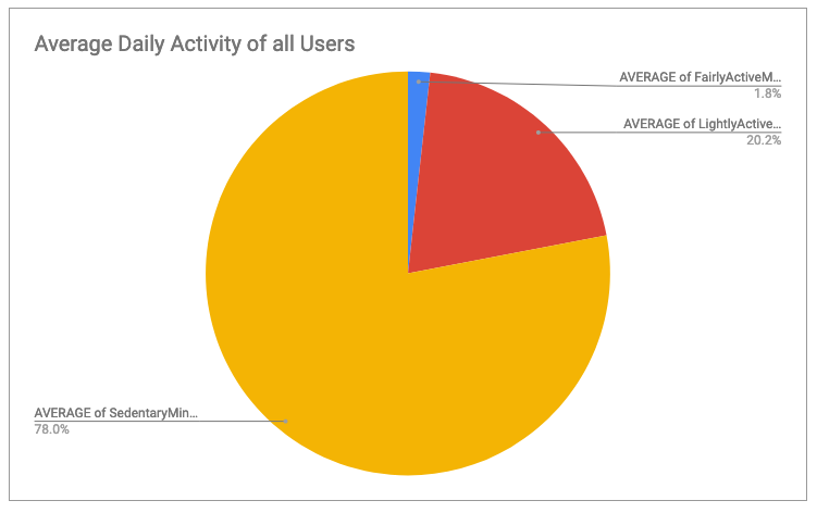
- Most users spent the majority of their time each day sedentary – over 78% of their day. Very Active minutes made up such a small percentage of daily time that it was not shown in this pie chart. Calculations and chart, Google Sheets.
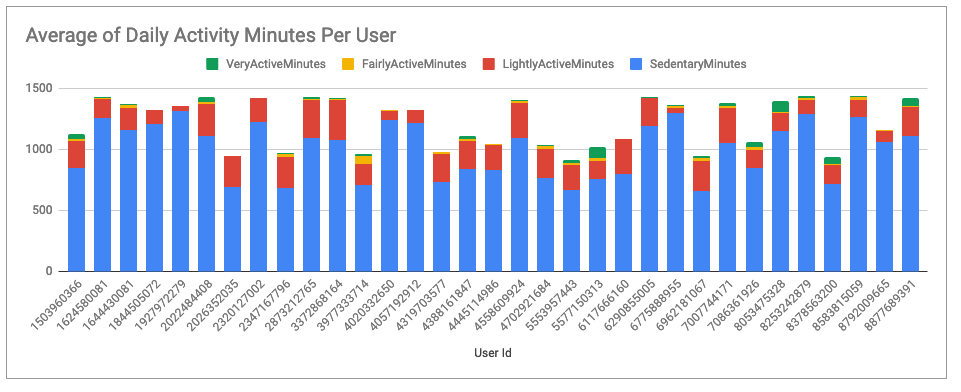
- Here is another look at activity levels per user. As you can see, each user has a significant amount of sedentary time on average. Calculations and chart, Google Sheets.
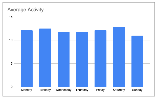
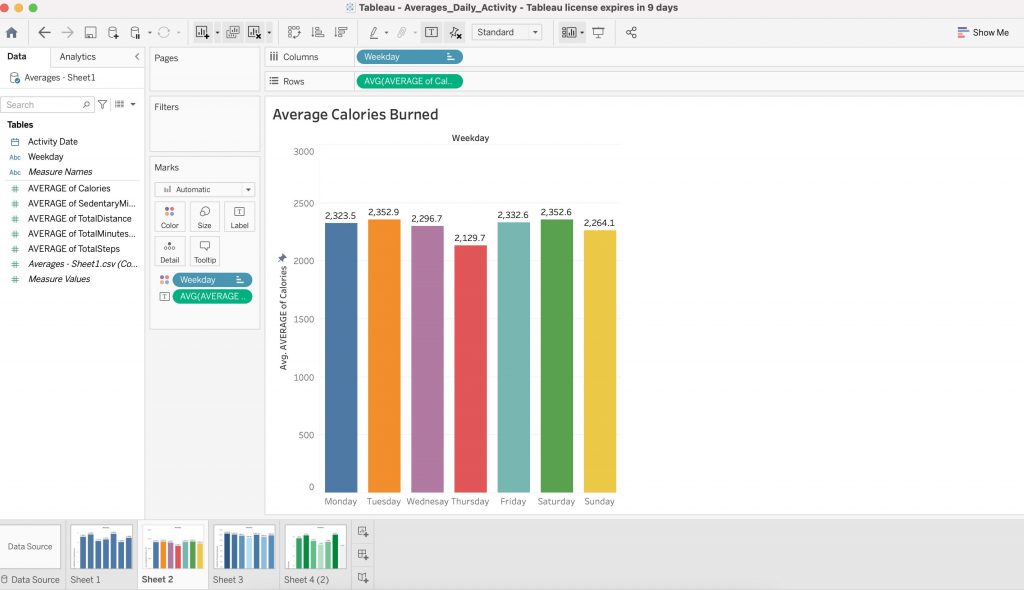
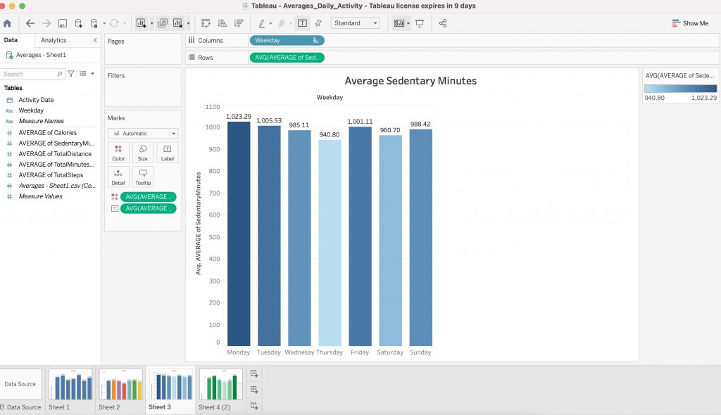
- This chart shows average activity during the week. As you can see, users were most active on Tuesdays and Saturdays and least active on Sundays, Wednesdays and Thursdays. Calculation and chart, Google Sheets.
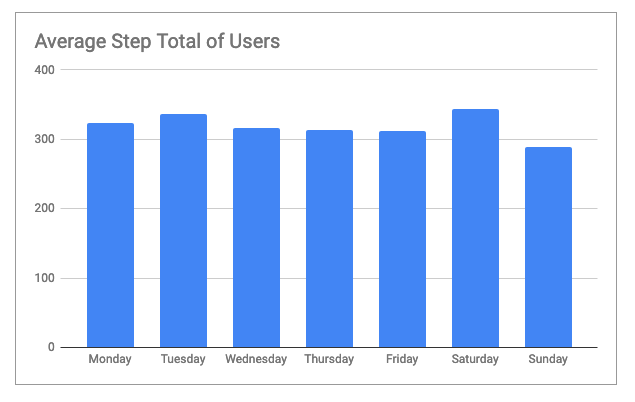
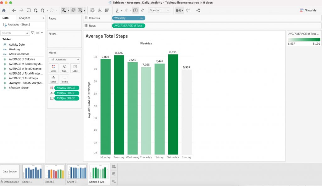
- This chart shows the average step totals for all users. As you can see, step totals were highest on Tuesdays and Saturdays and lowest on Sundays, Thursdays and Wednesdays. Calculations and chart, Google Sheets.
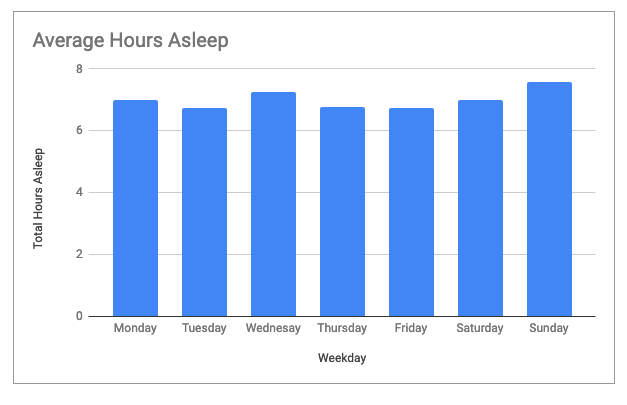
- This chart shows the average hours asleep for all users. As you can see, users slept the most hours on Sundays and Wednesdays which correlates to their activity levels. The lowest hours of sleep per day were on Tuesdays and Fridays. Calculations and chart, Google Sheets.
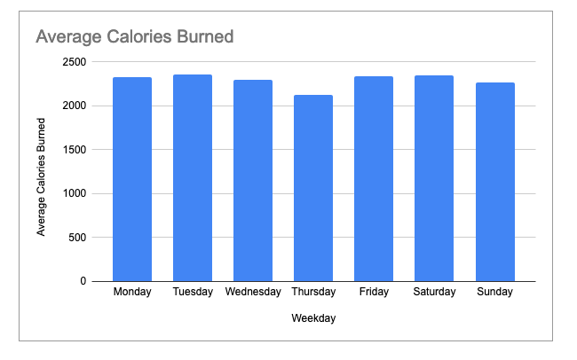
- As you can see from this chart, users burned the most calories on Tuesdays and Saturdays. Users burned the least amount of calories on Thursdays and Sundays. Calculations and chart, Google Sheets.
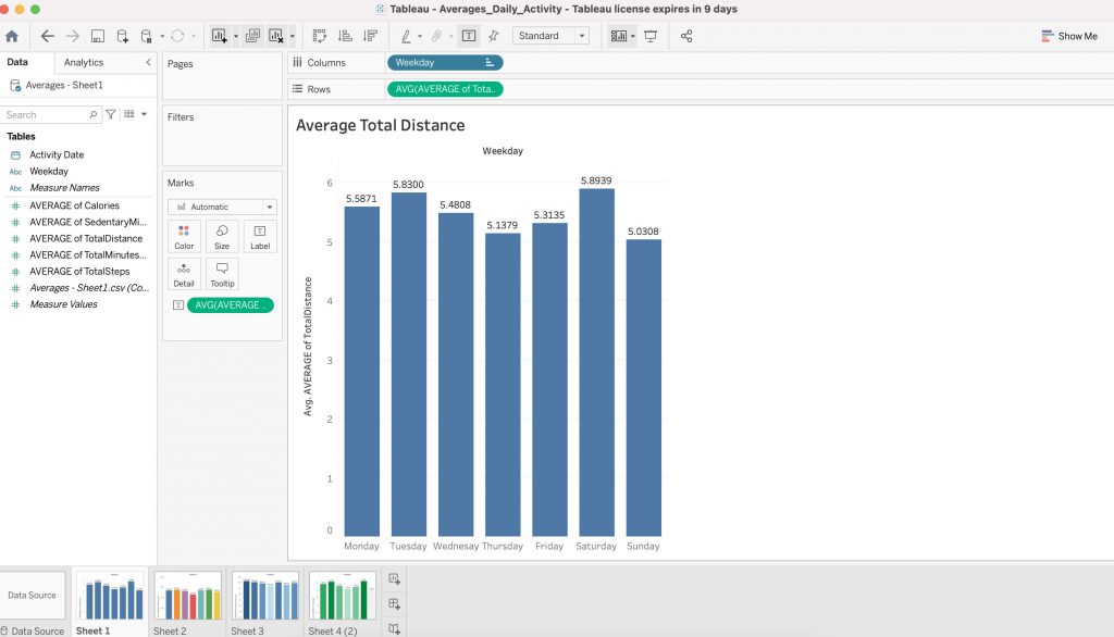
- The same calculations were visualised using Tableau below.
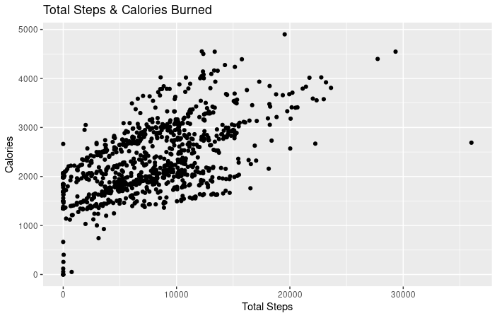
- As you can see from this chart, there is a positive correlation between total steps and calories burned. Chart and calculations, R Studio.
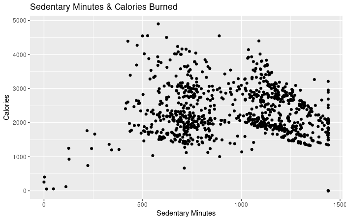
- As you can see from this chart, there is a negative correlation between sedentary minutes and calories burned (meaning the more sedentary minutes, the less calories are burned). Calculations and chart, R Studio.
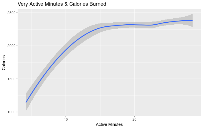
- As you can see from this chart, there is a positive correlation between very active minutes and calories burned. Calculations and chart, R Studio.
- As you can see from this chart, there is a positive correlation between the tracker distance and total steps. Calculations and chart, R Studio.
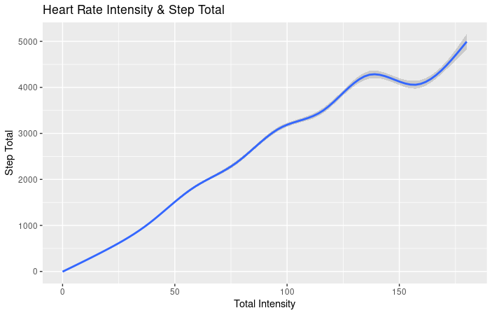
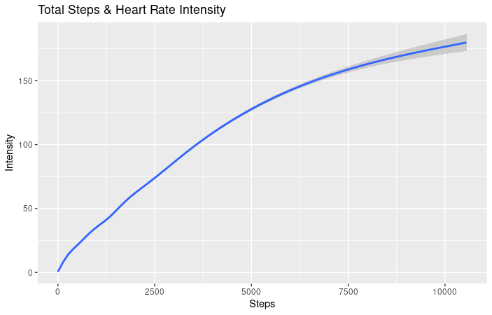
- As you can see from this chart, there is a positive correlation between heart rate intensity and step total. Calculations and chart, R Studio.
- As you can see from this chart, there is a positive correlation between total steps and heart rate intensity. Chart and calculations, R Studio.
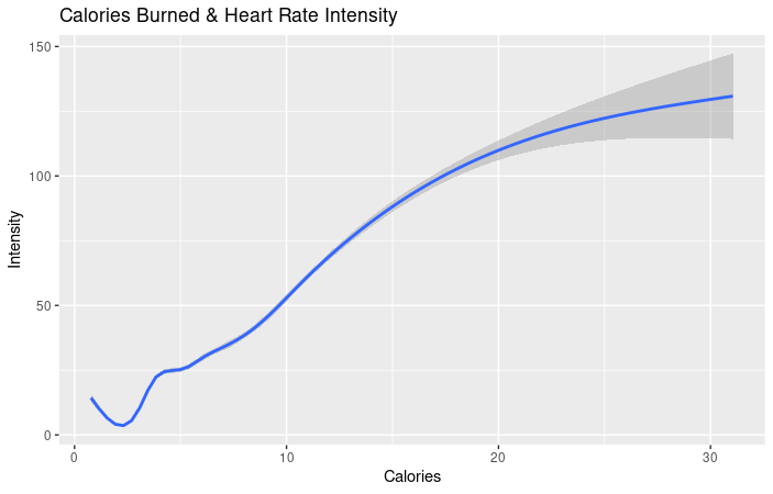
- As you can see from this chart, there is a positive correlation between calories burned and heart rate intensity. Calculations and chart, R Studio.
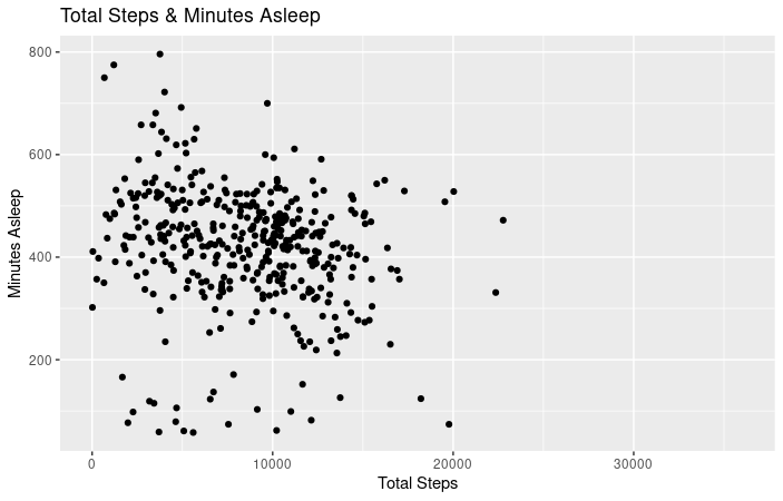
- As you can see from this chart, there is a negative correlation between total minutes asleep and total steps. The more the user sleeps, the less steps are taken. Calculations and chart, R Studio.
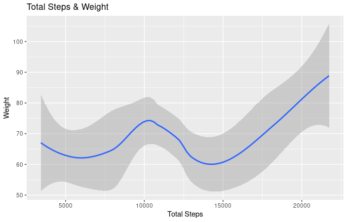
- As you can see from this chart, there seems to be positive correlation between an increase in total steps and weight. Looking at this data, one could assume that the weight increase is due to athleticism and muscular build. If the user is totalling more steps and there is an increase in weight, an assumption could be made that there is an increase in muscle mass. Please note, only 8 of the 33 users recorded weight and the reporting was sporadic. Calculations and chart, R Studio.
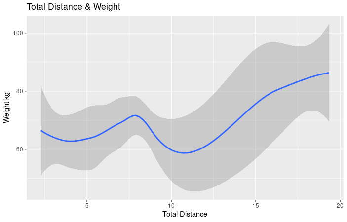
- As you can see from this chart, as total distance increases so does weight. As per the chart above, an assumption can be made that there is a relationship between total steps and weight due to athleticism and muscular build. Calculations and chart, R Studio.
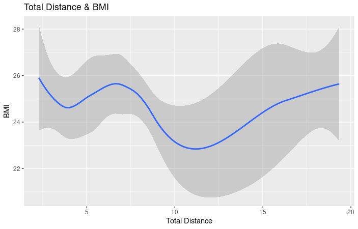
- As you can see from this chart, as total distance increases so does BMI. Again, we can assume that the BMI and distance increase are due to athleticism and muscular body composition. Calculations and chart, R Studio.
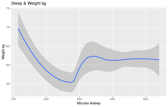
- As you can see from this chart, there is a negative correlation between weight and minutes asleep. The more minutes the user spent asleep, the weight decreased, rose and then levelled out. This could be attributed to a lack of user input for both sleep and weight. But it can also signify the healthy benefits of sleep. Calculations and chart, R Studio.
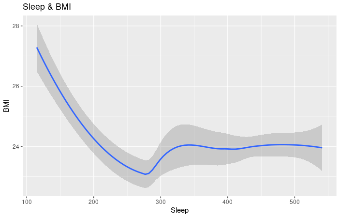
- As you can see in this chart, there is a negative correlation between sleep and BMI. As sleep increases, BMI decreases. This could be attributed to a lack of user input for both sleep and BMI. But it can also signify the healthy benefits of sleep. Calculations and chart, R Studio.
Conclusion
Summary: From the data, we can clearly see basic correlations: the amount of activity and the intensity of activity has a direct effect on calories burned and heart rate. We can also see some overall weekly trends, such as high activity on Tuesday and Saturday and low activity on Sunday and Wednesday. We can also tell from the weight and BMI data, that longer distances and increased active minutes is attributed to users with higher BMI and weight, but is manually inputted so it was only entered by 8 users. Sleep data shows that no users slept more than 8 hours and this data is also unreliable as many users did not wear their Fitbit at night. Overall, device usage decreased over the 30-day period.
1. During which time of day were the users most sedentary? Most active? Why?
On average, users were most active daily during 5pm-7pm. There was no recorded activity prior to 4am, but activity begins to increase after 5am and peaking at 11am before it begins to drop off until an increase after 3pm. As for why, this is in keeping with a typical work-day. Some users may exercise before work, then in the middle of the day, stay still until after 3pm when again, users begin to leave work and may exercise between the hours of 5pm-7pm.
2. During which time of the week were the users most active? Most sedentary? Why?
On average, users were most active on Tuesday and Saturday and most sedentary on Sunday, Wednesday and Thursday. Saturday tends to be a busy day, whereas Sunday also tends to be a day where most people relax and unwind.
3. What were the sleep trends? Which days had the most sleep minutes? Why?
On average, users slept the most hours on Sunday and Wednesday which lines up with their sedentary minutes. Users slept the least amount of time on Tuesday and Friday.
4. Was there a correlation between steps and calories?
Yes, the data showed there was a positive correlation between steps and calories, between total distance and calories and between intensity and calories.
5. Was there a correlation between sleep and calories?
Yes, there was a negative correlation between sedentary minutes and calories as well as sleep and calories. The more a user slept, the less calories were burned.
6. Is there a correlation between steps and sleep?
Yes, there is a negative correlation between steps and sleep. On average users who got more sleep, totalled less steps.
7. How did users report data? Automatically? Inputted?
The data that was recorded automatically such as distance, steps, calories, intensity and minutes was recorded as long as the user wore the Fitbit. Data such as weight and BMI was inputted manually which is why this data was not recorded consistently for all users. Sleep was also not consistently recorded which might mean that users removed their device during the night.
8. User weak points? Strong points?
Users were very unlikely to record data that required manual input, such as weight, and to wear the device at night to measure sleep.
9. Why do some users have more data than others?
Stated above, due to manual entry and Fitbit wear.
Overall, the data was not large or comprehensive enough to make a reliable analysis. But looking at this small sample size, did provide some valuable insights into how users interact with their wearble fitness device. For example, overall usage went down over the course of the thirty-day period. Also, users were highly unlikely to input any manual data or wear their device to sleep. The data did not disclose the sex or age of the users which would have been beneficial for this analysis.
Looking at this data, Bellabeat is well positioned to market the Leaf device as easy-to-wear with a battery-life of six months. This ease and versatility of wear (as a bracelet, necklace or clip) combined with the battery life, would most likely mean that users would record more consistent and reliable data. Also, the more automatic data Bellabeat can capture the better as we can see from this dataset, users were unlikely to manually track their weight.
Calculations & Raw Data
All files added to Google Sheets except the following files which were opened in Excel and BigQuery (SQL):Heartrate_seconds_merged (opened in excel)
minuteCaloriesNarrow_merged.csv (opened in excel)
minuteIntensitiesNarrow_merged.csv (opened in excel)
minuteMETsNarrow_merged.csv (opened in excel)
minuteSleep_merged.csv (opened in excel)
minuteStepsNarrow_merged.csv (opened in excel)
minuteStepsWide_merged.csv (opened in excel)Cleaning Data
Major formatting issue across all files – date- time stamp included in one column as string. Formatting is inaccurate for each user – some use 24 hours, others use AM/PM. Easily Changed time to 24-hour – in Google Sheets
Larger files were cleaned in R Studio
30-days of weight data only available for two users
Aggregated data manually in sheets: daily activity; sleep; weight to examine correlations. Very small sample size.
DailyActivity_merged.csv; 14 users have missing data – entered as 0 across all fields.
1503960366 – user does not have any values for 5/12/2016 in daily_activity_merged
1644430081 – user does not have data for 5/12/2016
1844505072 – user does not have any data for 4/24/2016 – 4/27/2016; 5/2/2016; 5/7/2016 – 5/12/2016 (entered as 0)
1927972279 – user does not have any data for 4/16/2016 – 4/17/2016; 4/19/2016-4/21/2016; 4/27/2016; 4/29/2016-4/30/2016; 5/5/2016; 5/8/2016-5/12/2016
3977333714 – user does not have any data for 5/12/2016
4020332650 – user does not have any data for 4/19/2016 – 5/1/2016
5577150313 – user missing data for 5/12/2016
6117666160 – user missing data for 4/12/2016 – 4/14/2016; 4/25/2016; 5/3/2016; 5/10/2016-5/12/2016;
6290855005 – user missing data for 4/21/2016; 4/23/2016; 4/26/2016; 4/29/2016; 5/10/2016 – 5/12/2016
6775888955 – user missing data for 4/12/2016; 4/19/2016; 4/21/2016; 4/23/2016; 4/27/2016; 4/29/2016; 5/2/2016; 5/4/2016; 5/5/2016; 5/8/2016-5/12/2016
7007744171 – user missing data for 5/4/2016; 5/7/2016-5/12/2016
7086361926 – user missing data for 4/17/2016
8253242879 – use missing data for 4/30/2016 – 5/12/2016
8792009665 – user missing data for 4/17/2016-4/19/2016; 4/25/2016; 5/5/2016 – 5/12/2016
Sleepday_merged:
only had data for 24 users; many records incomplete
1503960366 – missing data for 5/12/2016
1644430081 – only 4 entries out of 30
1844505072 – only 3 entries out of 30
1927972279 – only 5 entries out of 30
2320127002 – only 1 entry out of 30
2347167796 – only 15 entries out of 30
3977333714 – missing 2 entries
4020332650 – only 8 entries out of 30
4319703577 – only missing 2 entries
4388161847 – missing 3 entries
4558609924 – only 5 entries out of 30
5577150313 – missing 5 entries
6117666160 – missing 7 entries
6775888955 – only 3 entries out of 30
7007744171 – only 2 entries out of 30
8053475328 – only 3 entries out of 30
Added day of the week to all tables.
Added sleepday_merged.csv (and DailyActivity_merged.csv to BigQuery SQL
Performed the following join to aggregate the data:
SELECT a.ActivityDate, a.ID, a.TotalSteps, a.TotalDistance, a.VeryActiveDistance, a.ModeratelyActiveDistance, a.LightActiveDistance, a.SedentaryActiveDistance, a.VeryActiveMinutes, a.FairlyActiveMinutes, a.LightlyActiveMinutes, a.SedentaryMinutes, a.Calories, s.SleepDay, s.TotalMinutesAsleep
FROM `capstone-316723.fitbit_data.daily_activity` as a
LEFT JOIN `capstone-316723.fitbit_data.sleep` as s
ON a.Id = s.Id and a.ActivityDate = s.SleepDay
Formatted time-date stamp to 24-hour in hourlyintensities_merged.csv and hourlysteps_merged.csv. Added both files to BigQuery/SQL. Joined all data.
SELECT a.Id, a.ActivityHour, a.StepTotal, s.Id, s.ActivityHour, s.TotalIntensity, s.AverageIntensity
FROM `capstone-316723.fitbit_data.hourlysteps` as a
LEFT JOIN `capstone-316723.fitbit_data.hourlyintensities` as s
ON a.Id = s.Id and a.ActivityHour = s.ActivityHour
Formatted time-date stamp to 24-hour in minuteCalorieswide_merged.csv and minuteIntensitiesWide_merged.csv. Added both files to BigQuery/SQL. Joined all data.
SELECT *
FROM `capstone-316723.fitbit_data.minutecalories` as a
LEFT JOIN `capstone-316723.fitbit_data.minuteintensities` as s
ON a.Id = s.Id and a.ActivityHour = s.ActivityHour
SELECT ActivityHour, AVG(TotalIntensity) as Average_Intensity
FROM `capstone-316723.fitbit_data.hourlyintensities`
GROUP BY ActivityHour
For most of the calculations, pivot tables in Google Sheets and R Studio used.
To start with, I uploaded mergedSleep_merged.csv into R Studio to explore the file.
install.packages(“tidyverse”)
library(tidyverse)
install.packages(“skimr”)
library(skimr)
install.packages(“janitor”)
library(janitor)
installl.packages(“here”)
library(here)
install.packages(“psych”)
library(psych)
- Uploaded file into workspace
- > read_csv(“heartrate_seconds_merged.csv”)
── Column specification ────────────────────────────────────────────────────────────────────────────────────────
cols(
Id = col_double(),
Time = col_character(),
Value = col_double()
)
|===================================================================================================| 100% 85 MB
# A tibble: 2,483,658 x 3
Id Time Value
<dbl> <chr> <dbl>
1 2022484408 4/12/2016 7:21:00 AM 97
2 2022484408 4/12/2016 7:21:05 AM 102
3 2022484408 4/12/2016 7:21:10 AM 105
4 2022484408 4/12/2016 7:21:20 AM 103
5 2022484408 4/12/2016 7:21:25 AM 101
6 2022484408 4/12/2016 7:22:05 AM 95
7 2022484408 4/12/2016 7:22:10 AM 91
8 2022484408 4/12/2016 7:22:15 AM 93
9 2022484408 4/12/2016 7:22:20 AM 94
10 2022484408 4/12/2016 7:22:25 AM 93
# … with 2,483,648 more rows
- heart <- read.csv(“heartrate_seconds_merged.csv”, stringsAsFactors = TRUE)
- head(heart)
Id Time Value
1 2022484408 4/12/2016 7:21:00 AM 97
2 2022484408 4/12/2016 7:21:05 AM 102
3 2022484408 4/12/2016 7:21:10 AM 105
4 2022484408 4/12/2016 7:21:20 AM 103
5 2022484408 4/12/2016 7:21:25 AM 101
6 2022484408 4/12/2016 7:22:05 AM 95
- summary(heart)
Id Time Value
Min. :2.022e+09 4/20/2016 11:52:15 AM: 12 Min. : 36.00
1st Qu.:4.388e+09 4/20/2016 12:11:10 PM: 12 1st Qu.: 63.00
Median :5.554e+09 4/20/2016 2:59:20 PM : 12 Median : 73.00
Mean :5.514e+09 4/15/2016 8:46:50 AM : 11 Mean : 77.33
3rd Qu.:6.962e+09 4/15/2016 9:27:50 AM : 11 3rd Qu.: 88.00
Max. :8.878e+09 4/15/2016 9:37:50 AM : 11 Max. :203.00
(Other) :2483589
NOTE: tried to plot data with this file, but it was too large. The system could not handle the input.
- Uploaded the file into workspace.
- > read_csv(“DailyActivity_merged.csv”)
── Column specification ──────────────────────────────────────────────────────
cols(
Id = col_double(),
ActivityDate = col_character(),
TotalSteps = col_double(),
TotalDistance = col_double(),
TrackerDistance = col_double(),
LoggedActivitiesDistance = col_double(),
VeryActiveDistance = col_double(),
ModeratelyActiveDistance = col_double(),
LightActiveDistance = col_double(),
SedentaryActiveDistance = col_double(),
VeryActiveMinutes = col_double(),
FairlyActiveMinutes = col_double(),
LightlyActiveMinutes = col_double(),
SedentaryMinutes = col_double(),
Calories = col_double()
)
# A tibble: 940 x 15
Id ActivityDate TotalSteps TotalDistance TrackerDistance
<dbl> <chr> <dbl> <dbl> <dbl>
1 1503960366 4/12/2016 13162 8.5 8.5
2 1503960366 4/13/2016 10735 6.97 6.97
3 1503960366 4/14/2016 10460 6.74 6.74
4 1503960366 4/15/2016 9762 6.28 6.28
5 1503960366 4/16/2016 12669 8.16 8.16
6 1503960366 4/17/2016 9705 6.48 6.48
7 1503960366 4/18/2016 13019 8.59 8.59
8 1503960366 4/19/2016 15506 9.88 9.88
9 1503960366 4/20/2016 10544 6.68 6.68
10 1503960366 4/21/2016 9819 6.34 6.34
# … with 930 more rows, and 10 more variables:
# LoggedActivitiesDistance <dbl>, VeryActiveDistance <dbl>,
# ModeratelyActiveDistance <dbl>, LightActiveDistance <dbl>,
# SedentaryActiveDistance <dbl>, VeryActiveMinutes <dbl>,
# FairlyActiveMinutes <dbl>, LightlyActiveMinutes <dbl>,
# SedentaryMinutes <dbl>, Calories <dbl>
- activity <- read.csv(“DailyActivity_merged.csv”, stringsAsFactors = TRUE)
- dim(activity)
[1] 940 15
- colnames(activity)
[1] “Id” “ActivityDate”
[3] “TotalSteps” “TotalDistance”
[5] “TrackerDistance” “LoggedActivitiesDistance”
[7] “VeryActiveDistance” “ModeratelyActiveDistance”
[9] “LightActiveDistance” “SedentaryActiveDistance”
[11] “VeryActiveMinutes” “FairlyActiveMinutes”
[13] “LightlyActiveMinutes” “SedentaryMinutes”
[15] “Calories”
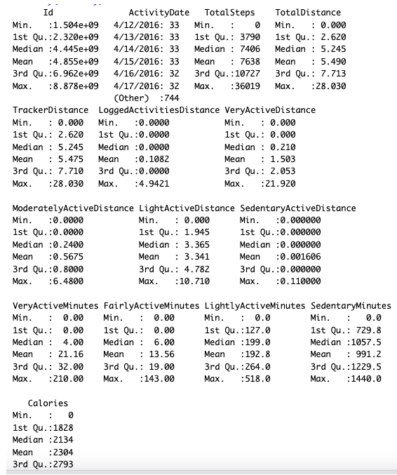
- summary(activity)
7. head(activity)

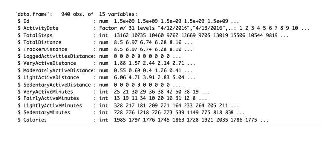
8. str(activity)
- activity %>% group_by(Id) %>%
drop_na() %>%
summarize(mean_total_steps=mean(TotalSteps))
Id mean_total_steps
<dbl> <dbl>
1 1503960366 12117.
2 1624580081 5744.
3 1644430081 7283.
4 1844505072 2580.
5 1927972279 916.
6 2022484408 11371.
7 2026352035 5567.
8 2320127002 4717.
9 2347167796 9520.
10 2873212765 7556.
# … with 23 more rows
2. glimpse(mean_total_steps)
3. colnames(mean_total_steps) <- c(“Id”,”Steps”)
# A tibble: 6 x 2
Id Steps
<dbl> <dbl>
1 1503960366 12117.
2 1624580081 5744.
3 1644430081 7283.
4 1844505072 2580.
5 1927972279 916.
6 2022484408 11371.
ggplot(data=activity)+ geom_point(mapping=aes(x=TotalSteps,y=Calories))
ggplot(data=activity)+ geom_smooth(mapping=aes(x=TotalSteps,y=Calories))
ggplot(data=activity)+ geom_point(mapping=aes(x=SedentaryMinutes,y=Calories))
ggplot(data=activity)+ geom_smooth(mapping=aes(x=SedentaryMinutes,y=Calories))
ggplot(data=activity)+geom_point(mapping=aes(x=TrackerDistance,y=TotalSteps))
ggplot(data=activity)+geom_point(mapping=aes(x=VeryActiveMinutes,y=Calories))
- Uploaded the file into the workspace.
- read_csv(“minuteSleep_merged.csv”)
- sleep <- read.csv(“minuteSleep_merged.csv”, stringsAsFactors = TRUE)
- dim(sleep)
- [1] 188521 4
- colnames(sleep)
- [1] “Id” “date” “value” “logId”
- summary(sleep$value)
- Min. 1st Qu. Median Mean 3rd Qu. Max.
- 1.000 1.000 1.000 1.096 1.000 3.000
- head(sleep)
Id date value logId
1 1503960366 4/12/2016 2:47:30 AM 3 11380564589
2 1503960366 4/12/2016 2:48:30 AM 2 11380564589
3 1503960366 4/12/2016 2:49:30 AM 1 11380564589
4 1503960366 4/12/2016 2:50:30 AM 1 11380564589
5 1503960366 4/12/2016 2:51:30 AM 1 11380564589
6 1503960366 4/12/2016 2:52:30 AM 1 11380564589
- glimpse(sleep)
Rows: 188,521
Columns: 4
$ Id <dbl> 1503960366, 1503960366, 1503960366, 1503960366, 1503960366, 15…
$ date <fct> 4/12/2016 2:47:30 AM, 4/12/2016 2:48:30 AM, 4/12/2016 2:49:30 …
$ value <int> 3, 2, 1, 1, 1, 1, 1, 2, 2, 2, 3, 3, 3, 3, 3, 2, 1, 1, 1, 1, 1,…
$ logId <dbl> 11380564589, 11380564589, 11380564589, 11380564589, 1138056458…
- Upload heartrate_seconds_merged.csv
- read_csv(“heartrate_seconds_merged.csv”)
Id Time Value
<dbl> <chr> <dbl>
1 2022484408 4/12/2016 7:21:00 AM 97
2 2022484408 4/12/2016 7:21:05 AM 102
3 2022484408 4/12/2016 7:21:10 AM 105
4 2022484408 4/12/2016 7:21:20 AM 103
5 2022484408 4/12/2016 7:21:25 AM 101
6 2022484408 4/12/2016 7:22:05 AM 95
7 2022484408 4/12/2016 7:22:10 AM 91
8 2022484408 4/12/2016 7:22:15 AM 93
9 2022484408 4/12/2016 7:22:20 AM 94
10 2022484408 4/12/2016 7:22:25 AM 93
# … with 2,483,648 more rows
- heart <- read.csv(“heartrate_seconds_merged.csv”, stringsAsFactors = TRUE)
- head(heart)
Id Time Value
1 2022484408 4/12/2016 7:21:00 AM 97
2 2022484408 4/12/2016 7:21:05 AM 102
3 2022484408 4/12/2016 7:21:10 AM 105
4 2022484408 4/12/2016 7:21:20 AM 103
5 2022484408 4/12/2016 7:21:25 AM 101
6 2022484408 4/12/2016 7:22:05 AM 95
3. dim(heart)
[1] 2483658 3
4. summary(heart)
Id Time Value
Min. :2.022e+09 4/20/2016 11:52:15 AM: 12 Min. : 36.00
1st Qu.:4.388e+09 4/20/2016 12:11:10 PM: 12 1st Qu.: 63.00
Median :5.554e+09 4/20/2016 2:59:20 PM : 12 Median : 73.00
Mean :5.514e+09 4/15/2016 8:46:50 AM : 11 Mean : 77.33
3rd Qu.:6.962e+09 4/15/2016 9:27:50 AM : 11 3rd Qu.: 88.00
Max. :8.878e+09 4/15/2016 9:37:50 AM : 11 Max. :203.00
(Other) :2483589
- Uploaded file.
- read_csv(“activitysleepmerged.csv”)
- activesleep <- read.csv(“activitysleepmerged.csv”, stringsAsFactors = TRUE)
- head(activesleep)
- ActivityDate ID TotalSteps TotalDistance VeryActiveDistance1 2016-05-01 1624580081 36019 28.03 21.922 2016-04-14 1644430081 11037 8.02 0.363 2016-04-19 1644430081 11256 8.18 0.364 2016-04-28 1644430081 9405 6.84 0.205 2016-04-30 1644430081 18213 13.24 0.636 2016-05-03 1644430081 12850 9.34 0.72ModeratelyActiveDistance LightActiveDistance SedentaryActiveDistance1 4.19 1.91 0.022 2.56 5.10 0.003 2.53 5.30 0.004 2.32 4.31 0.005 3.14 9.46 0.006 4.09 4.54 0.00VeryActiveMinutes FairlyActiveMinutes LightlyActiveMinutes SedentaryMinutes1 186 63 171 10202 5 58 252 11253 5 58 278 10994 3 53 227 11575 9 71 402 8166 10 94 221 1115TotalMinutesAsleep1 NA2 NA3 NA4 NA5 1246 NAggplot(data=activesleep)+geom_smooth(mapping=aes(x=TotalSteps,y=TotalMinutesAsleep))
- Uploaded file
- read_csv(“minuteintensities.csv”)
- intense <- read.csv(“minuteintensities.csv”, stringsAsFactors = TRUE)
- head(intense)
- ggplot(data=intense)+
geom_smooth(mapping=aes(x=Total,y=TOTAL))+ labs(x=”Calories”,y=”Intensities”)
- read_csv(“hourlyintensities.csv”)
- hourly <- read.csv(“hourlyintensities.csv”, stringsAsFactors = TRUE)
- head(hourly)
- ggplot(data=hourly)+
geom_smooth(mapping=aes(x=StepTotal,y=TotalIntensity))+
labs(x=”Steps”,y=”Intensities”)
- read_csv(“heartrate_seconds_merged.csv”)
2. heartrate <- read.csv(“hourlyintensities.csv”, stringsAsFactors = TRUE)
3. head(heartrate)
4. summary(heartrate)
6. ggplot(data=heartrate)+ geom_smooth(mapping=aes(x=TotalIntensity,y=StepTotal))+ labs(x=”Total Intensity”,y=”Step Total”)
- read_csv(“merged.csv”)
- merged <- read.csv(“merged.csv”, stringsAsFactors = TRUE)
- ggplot(data=merged)+geom_smooth(mapping=aes(x=TotalSteps,y=Weightkg))+labs(x=”Total Steps”,y=”Weight”)
- ggplot(data=merged)+ geom_smooth(mapping=aes(x=TotalDistance,y=Weightkg))+ labs(x=”Total Distance”,y=”Weight kg”)
- ggplot(data=merged)+ geom_smooth(mapping=aes(x=TotalDistance,y=BMI))+ labs(x=”Total Distance”,y=”BMI”)
- ggplot(data=merged)+geom_smooth(mapping=aes(x=TotalMinutesAsleep,y=BMI))+ labs(x=”Sleep”,y=”BMI”)
- ggplot(data=merged)+ geom_smooth(mapping=aes(x=TotalMinutesAsleep,y=Weightkg))+ labs(x=”Minutes Asleep”,y=”Weight”)
- ggplot(data=merged)+ geom_smooth(mapping=aes(x=TotalMinutesAsleep,y=BMI))+ labs(x=”Minutes Asleep”,y=”BMI”)